import pandas as pd
from plotnine import *
from plotnine.layer import layer
from plotnine.stats.stat import stat
from plotnine.session import last_plotRecipe #2, geom_index() and geom_coordinates()
The Goal
In the last recipe, you should have seen and practiced how to write a compute function that can be used in a stat. Specifically, you defined group-wise computation by defining compute_group in your stat class. You specified that other behavior should be inherited from the more generic stat class. You improved the user interface for your stat by specifying which aesthetics must be provided by the user in REQUIRED_AES. Finally you wrote user-facing stat_* and geom_* classes based on the new stat and an existing geom.
In this next recipe, we’ll first see the creation of stat_index and geom_index, which can be used to label observations with their row numbers.
Along the way, we’ll contrast a new extension move - defining panel-wise instead of group-wise compute using compute_panel. Panel-wise computation (computing by facet) will be used in the two recipes that follow.
In the exercise for this recipe, you’ll create stat_coordinates and geom_coordinates, usable to mark points with their x and y coordinates.
Let’s get started! By the end of the exercise, we should be able to specify the plot below with the new geom_coordinates() function:
(
    ggplot(data=cars)
    + aes(x="speed", y="dist")
    + geom_point()
    + geom_coordinates(  # new function!
        ha="right",
        va="top",
        adjust_text={"arrowprops": {"arrowstyle": "-"}},
    )
)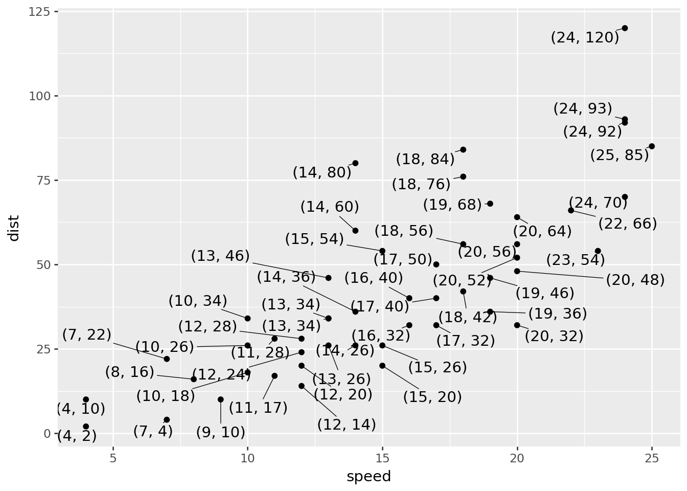
But, we’ll start by demonstrating how to annotate the observation index (row number) at x and y, defining the new extension function geom_index(). Then you’ll be prompted to define geom_coordinates() based on what you’ve learned.
Step 00: Loading packages and data
We’ll define the cars dataset as a DataFrame with columns speed and dist (equivalent to R’s built-in cars dataset).
import pandas as pd

cars = pd.read_csv("cars.csv")
cars| speed | dist | |
|---|---|---|
| 0 | 4 | 2 |
| 1 | 4 | 10 |
| 2 | 7 | 4 |
| 3 | 7 | 22 |
| 4 | 8 | 16 |
| 5 | 9 | 10 |
| 6 | 10 | 18 |
| 7 | 10 | 26 |
| 8 | 10 | 34 |
| 9 | 11 | 17 |
| 10 | 11 | 28 |
| 11 | 12 | 14 |
| 12 | 12 | 20 |
| 13 | 12 | 24 |
| 14 | 12 | 28 |
| 15 | 13 | 26 |
| 16 | 13 | 34 |
| 17 | 13 | 34 |
| 18 | 13 | 46 |
| 19 | 14 | 26 |
| 20 | 14 | 36 |
| 21 | 14 | 60 |
| 22 | 14 | 80 |
| 23 | 15 | 20 |
| 24 | 15 | 26 |
| 25 | 15 | 54 |
| 26 | 16 | 32 |
| 27 | 16 | 40 |
| 28 | 17 | 32 |
| 29 | 17 | 40 |
| 30 | 17 | 50 |
| 31 | 18 | 42 |
| 32 | 18 | 56 |
| 33 | 18 | 76 |
| 34 | 18 | 84 |
| 35 | 19 | 36 |
| 36 | 19 | 46 |
| 37 | 19 | 68 |
| 38 | 20 | 32 |
| 39 | 20 | 48 |
| 40 | 20 | 52 |
| 41 | 20 | 56 |
| 42 | 20 | 64 |
| 43 | 22 | 66 |
| 44 | 23 | 54 |
| 45 | 24 | 70 |
| 46 | 24 | 92 |
| 47 | 24 | 93 |
| 48 | 24 | 120 |
| 49 | 25 | 85 |
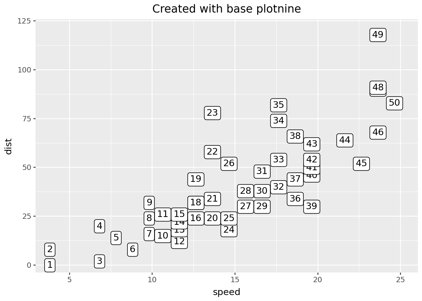
Step 0: use base plotnine to get the job done
It’s good idea to go through how you’d get things done without extension first, just using ‘base’ plotnine. The computational moves you make here can serve as a reference for building our extension function.
(
    ggplot(cars.assign(index=range(1, len(cars) + 1)))
    + aes(x="speed", y="dist", label="index")
    + geom_point()
    + geom_label(va="top", ha="right")
    + labs(title="Created with base plotnine")
)
TipPro tip. Use
ggplot.layer_data() to inspect plotnine’s internal data …
Use ggplot.layer_data() to inspect the render-ready data internal in the plot. Your stat will help prep data to look something like this.
last_plot().layer_data(i=1).head() # layer 2, with labels designated is of interest| x | y | label | PANEL | group | family | angle | lineheight | fontweight | color | size | fill | fontstyle | fontvariant | alpha | va | ha | |
|---|---|---|---|---|---|---|---|---|---|---|---|---|---|---|---|---|---|
| 0 | 4 | 2 | 1 | 1 | -1 | None | 0 | 1.2 | normal | black | 11 | white | normal | None | 1 | top | right |
| 1 | 4 | 10 | 2 | 1 | -1 | None | 0 | 1.2 | normal | black | 11 | white | normal | None | 1 | top | right |
| 2 | 7 | 4 | 3 | 1 | -1 | None | 0 | 1.2 | normal | black | 11 | white | normal | None | 1 | top | right |
| 3 | 7 | 22 | 4 | 1 | -1 | None | 0 | 1.2 | normal | black | 11 | white | normal | None | 1 | top | right |
| 4 | 8 | 16 | 5 | 1 | -1 | None | 0 | 1.2 | normal | black | 11 | white | normal | None | 1 | top | right |
Step 1: Define compute. Test.
Now you are ready to begin building your extension function. The first step is to define the compute that should be done under-the-hood when your function is used. We’ll define this in a function called compute_group_index(). The data input will look similar to the plot data. You will also need to include a scales argument, which plotnine uses internally.
Define compute
def compute_group_index(data, scales=None):
    return data.assign(label=range(1, len(data) + 1))
NoteYou may have noticed …
… the
scalesargument in the compute definition, which is used internally in plotnine. While it won’t be used in your test (up next), you do need it so that the computation will work in the plotnine setting.… that the compute function can only be used with data with variables
xandy. These aesthetic variable names, relevant for building the plot, are generally not found in the raw data inputs for the plot.… that the compute function adds a column of data called ‘label’ internally. This means that the stat can be used with geoms like
geom_textandgeom_labelwithout the user providing a label!
Test compute
# Test compute
(
    cars
    .rename(columns={"speed": "x", "dist": "y"})
    .pipe(compute_group_index)
    .head()
)| x | y | label | |
|---|---|---|---|
| 0 | 4 | 2 | 1 |
| 1 | 4 | 10 | 2 |
| 2 | 7 | 4 | 3 |
| 3 | 7 | 22 | 4 |
| 4 | 8 | 16 | 5 |
NoteYou may have noticed …
… that we prepare the data to have columns with names x and y before testing. Computation will fail if variables x and y are not present given the function’s definition. In a plotting setting, columns are renamed by mapping aesthetics, e.g. aes(x="speed", y="dist").
Step 2: Define new stat. Test.
Next, we define a new stat class — which will let us do computation under the hood while building our plot.
Define stat
from plotnine.stats.stat import stat

class stat_index(stat):  # <1> <2>
    REQUIRED_AES = {"x", "y"}
    DEFAULT_PARAMS = {"geom": "label"}

    def compute_group(self, data, scales):
        return compute_group_index(data)
NoteYou may have noticed…
… that the naming convention for the stat class uses snake_case. e.g.
stat_index.… that we inherit from the
statclass. In fact, your class is a subclass – you are inheriting class properties from plotnine’sstat.… that the
compute_group_indexfunction is called in thecompute_groupmethod. This means that data will be transformed group-wise by our compute definition – i.e. by categories if a categorical variable is mapped.… that setting
REQUIRED_AESto{"x", "y"}reflects the compute function’s requirements. SpecifyingREQUIRED_AESin your stat can improve your user interface. Standard plotnine error messages will issue if required aesthetics are not specified, e.g. “stat_index()requires the following missing aesthetics:x.”
Test stat
You can test out your stat by using it in plotnine geom_*() functions.
(
    ggplot(cars)
    + aes(x="speed", y="dist")
    + geom_point()
    + geom_text(stat=stat_index, ha="right", va="top")
    + labs(title="Testing stat_index")
)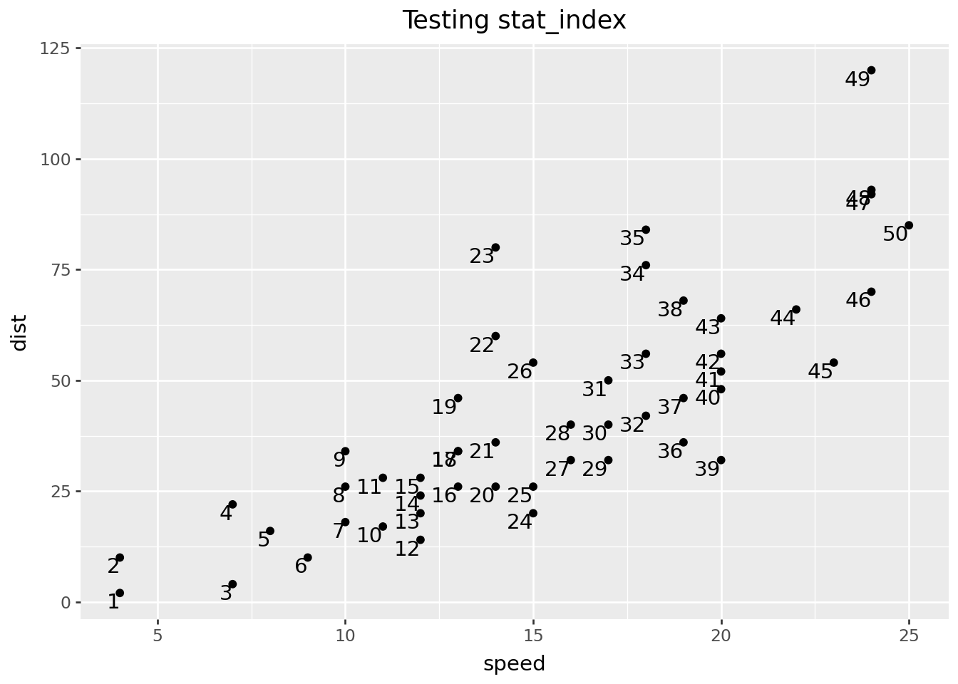
NoteYou may have noticed …
… that we pass the class stat_index to the stat argument. But you could also use the string! If you prefer, you could write geom_text(stat="index") which will direct to your new stat_index under the hood.
Test stat group-wise behavior
Test group-wise behavior by using a discrete variable with a group-triggering aesthetic like color, fill, or group, or by faceting.
last_plot() + aes(color="speed > 15")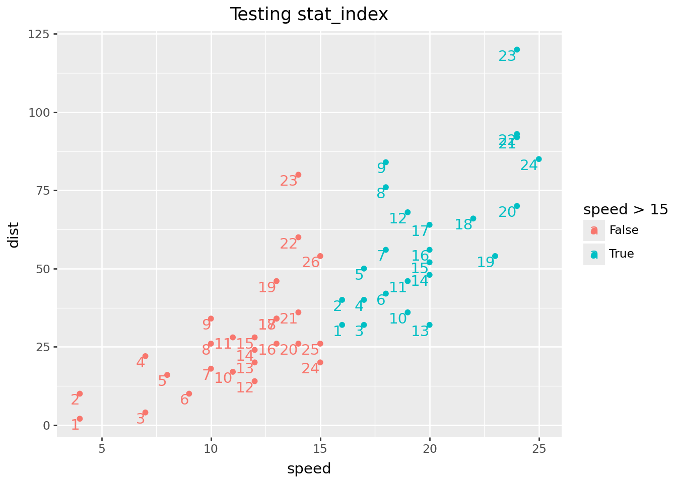
NoteYou may have noticed …
… that some indices change with color mapping. This is because compute is by group (compute_group is defined), so the index is within group.
Contrast this to the case where compute_panel is defined instead, which defines facet-wise computation.
class stat_index_panel(stat):
    REQUIRED_AES = {"x", "y"}
    DEFAULT_PARAMS = {"geom": "text"}

    def compute_panel(self, data, scales):
        return compute_group_index(data)

(
    ggplot(cars)
    + aes(x="speed", y="dist")
    + geom_point()
    + geom_text(stat=stat_index_panel, ha="right", va="top")
    + labs(title="Testing stat_index_panel")
    + aes(color="speed > 15")
)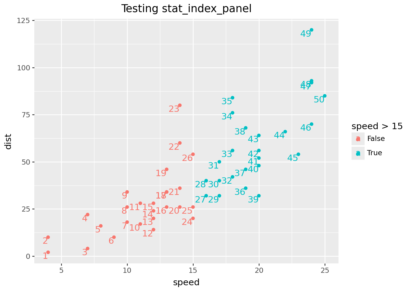
The indexing (row_numbers) are not computed within the T/F computed color variable speed > 15, but across the panel (facet).
The exercises that follow will specify compute_panel for the stat objects throughout.
TipPro tip: Think about an early exit (don’t define a user-facing function) …
You might be thinking, what we’ve done would already be pretty useful to me. Can I just use my stat as-is within geom_*() functions?
The short answer is ‘yes’! If you just want to use the stat yourself locally in a script, there might not be much reason to go on to Step 3, user-facing functions. But if you have a wider audience in mind, i.e. internal to organization or open sourcing in a package, probably a more succinct expression of what functionality you deliver will be useful - i.e. write the user-facing functions.
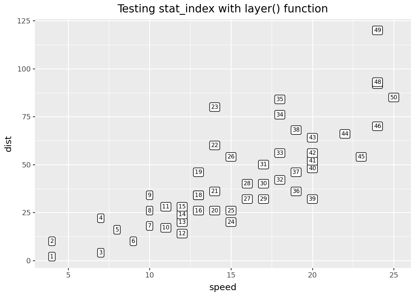
TipPro tip: consider using
layer() function to test instead of geom_*(stat=stat_new)
Instead of using a geom_*() function, you might prefer to use the layer() function in your testing step. Occasionally, you must go this route; for example, geom_vline() contains no stat argument, but you can use geom_vline in layer(). If you are teaching this content, using layer() may help you better connect this step with the next, defining the user-facing functions.
A test of stat_index using this method follows. You can see it is a little more verbose, as there is no default for the position argument, and setting the size must be handled with a little more care.
(
    ggplot(cars)
    + aes(x="speed", y="dist")
    + geom_point()
    + layer(
        geom=geom_label,
        stat=stat_index,
        position="identity",
        size=7,
    )
    + labs(title="Testing stat_index with layer() function")
)
Step 3: Define user-facing functions. Test.
In this next section, we define user-facing geom_* classes. In plotnine, creating a new geom is as simple as subclassing an existing geom and setting DEFAULT_PARAMS with your new stat.
Define geom_*() class
‘Most users are accustomed to adding geoms, not stats, when building up a plot.’ ggplot2: Elegant Graphics for Data Analysis.
Because plotnine users may be more accustomed to using layers that have the geom_ prefix, you might define a geom_ class with the same properties as the stat_. Here we subclass geom_label and set the default stat to "index".
class geom_index(geom_label):
    DEFAULT_PARAMS = {
        "stat": "index",
        "parse": False,
        "nudge_x": 0,
        "nudge_y": 0,
        "adjust_text": None,
        "format_string": None,
        "path_effects": None,
        "boxstyle": "round",
        "boxcolor": None,
        "label_padding": 0.25,
        "label_r": 0.25,
        "label_size": 0.7,
        "tooth_size": None,
    }
NoteYou may have noticed…
… that
geom_indexinherits fromgeom_label. This means the layer will render labels by default.… that
DEFAULT_PARAMSincludes all ofgeom_label’s parameters plus"stat": "index". In plotnine,DEFAULT_PARAMSis fully replaced (not merged) when subclassing, so every parent parameter must be redeclared.
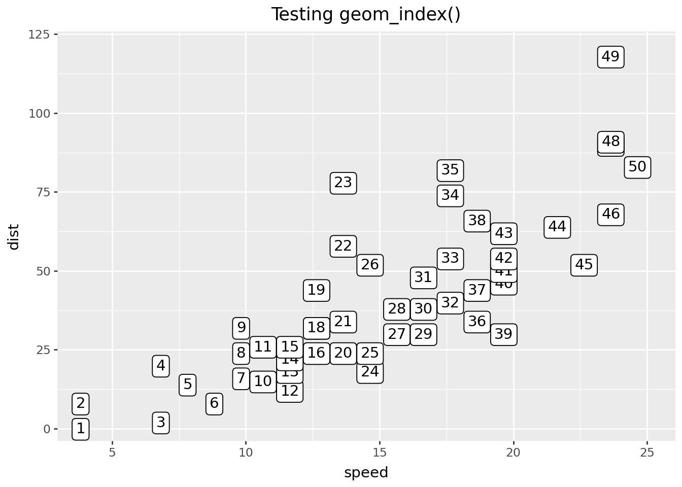
Test geom_index()
## Test user-facing
(
    ggplot(cars)
    + aes(x="speed", y="dist")
    + geom_point()
    + geom_index(ha="right", va="top")
    + labs(title="Testing geom_index()")
)
Test/Enjoy your user-facing functions
Test group-wise behavior
last_plot() + aes(color="speed > 15")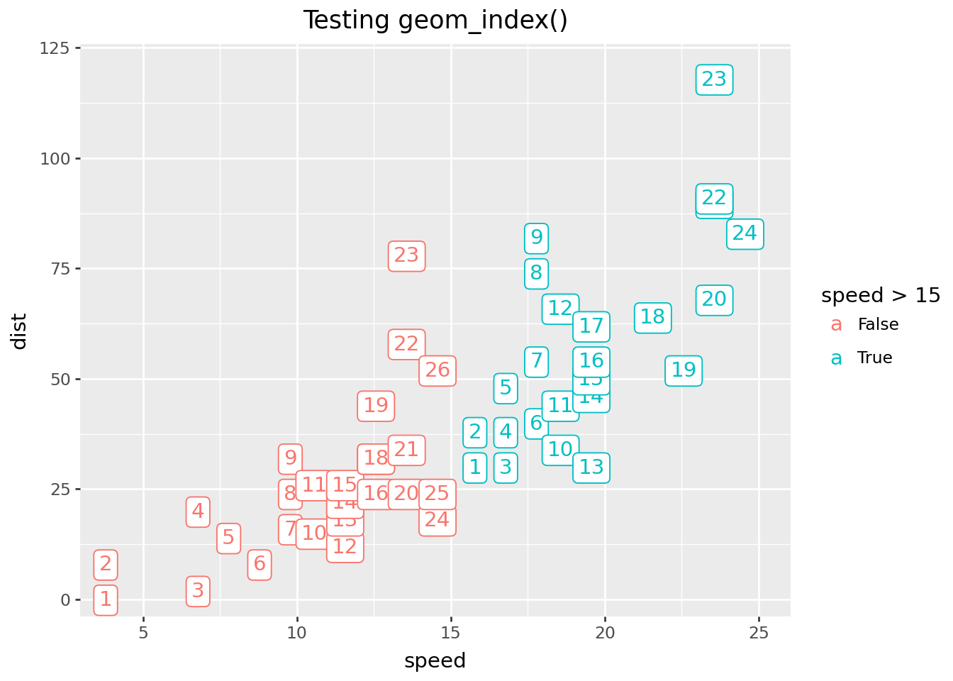
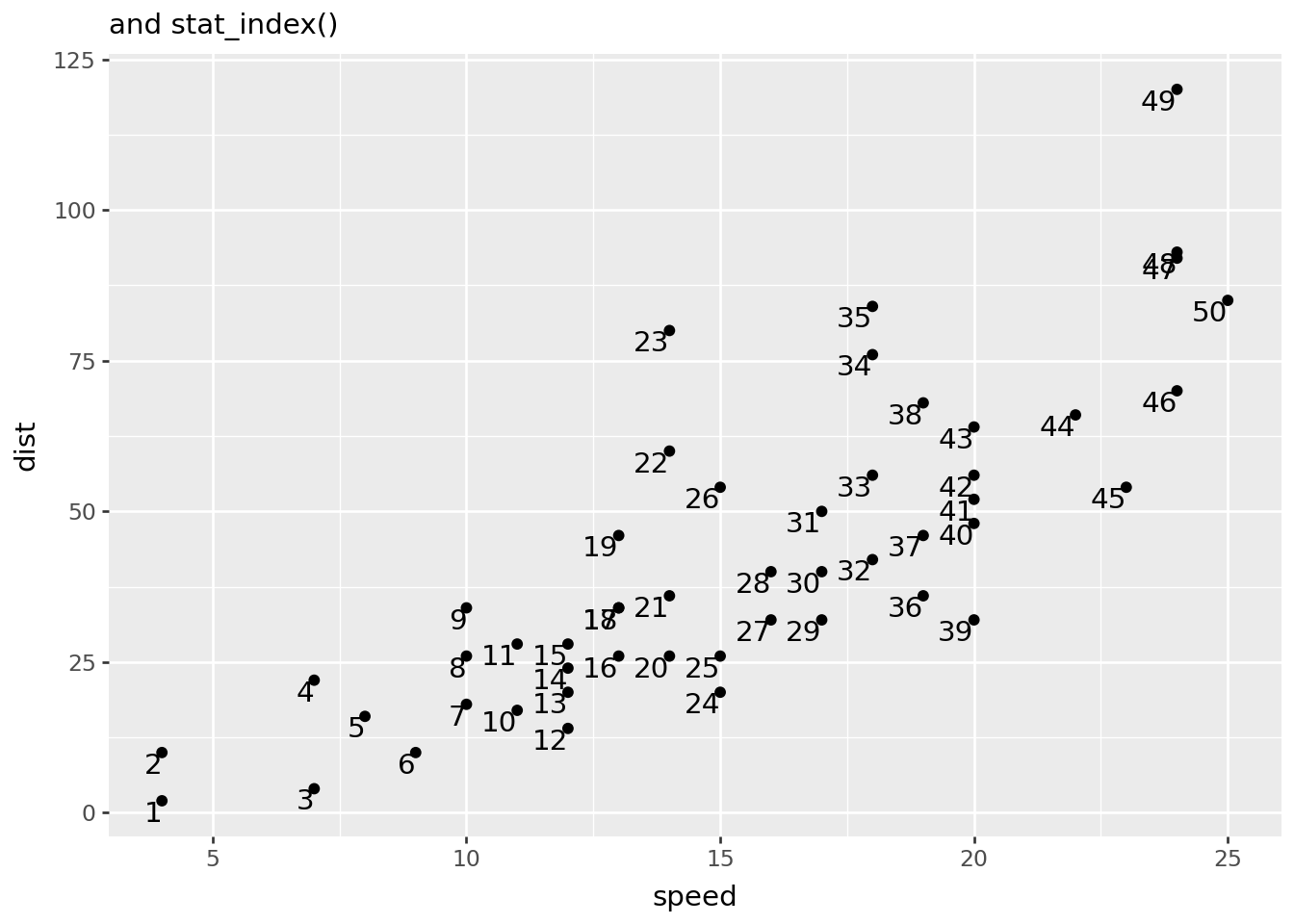
Use stat_*() function with another geom
(
    ggplot(cars)
    + aes(x="speed", y="dist")
    + geom_point()
    + stat_index(geom="text", ha="right", va="top")
    + labs(subtitle="and stat_index()")
)
Done! Time for a review.
Here is a quick review of the classes we’ve covered, dropping tests and discussion.
NoteReview
# Step 1. Define compute
def compute_group_index(data, scales=None):
    return data.assign(label=range(1, len(data) + 1))

# Step 2. Define stat
class stat_index(stat):
    REQUIRED_AES = {"x", "y"}
    DEFAULT_PARAMS = {"geom": "label"}

    def compute_group(self, data, scales):
        return compute_group_index(data)

# Step 3. Define geom
class geom_index(geom_label):
    DEFAULT_PARAMS = {
        "stat": "index",
        "parse": False,
        "nudge_x": 0,
        "nudge_y": 0,
        "adjust_text": None,
        "format_string": None,
        "path_effects": None,
        "boxstyle": "round",
        "boxcolor": None,
        "label_padding": 0.25,
        "label_r": 0.25,
        "label_size": 0.7,
        "tooth_size": None,
    }
Your Turn: write geom_coordinates()
Using the geom_index() Recipe #2 as a reference, try to create a stat_coordinates() class that labels points with their coordinates. You may also write a convenience geom_*() class.
Step 00: load libraries, data
Step 0: Use base plotnine to get the job done
Step 1: Write compute function. Test.
Step 2: Write stat.
Step 3: Write user-facing geom class.
Next up: Recipe 3 geom_bal_point() and geom_support()
In the next recipe, we’ll look at computation when we know we’ll be working with categorical variables, creating geom_bal_point() and geom_support().