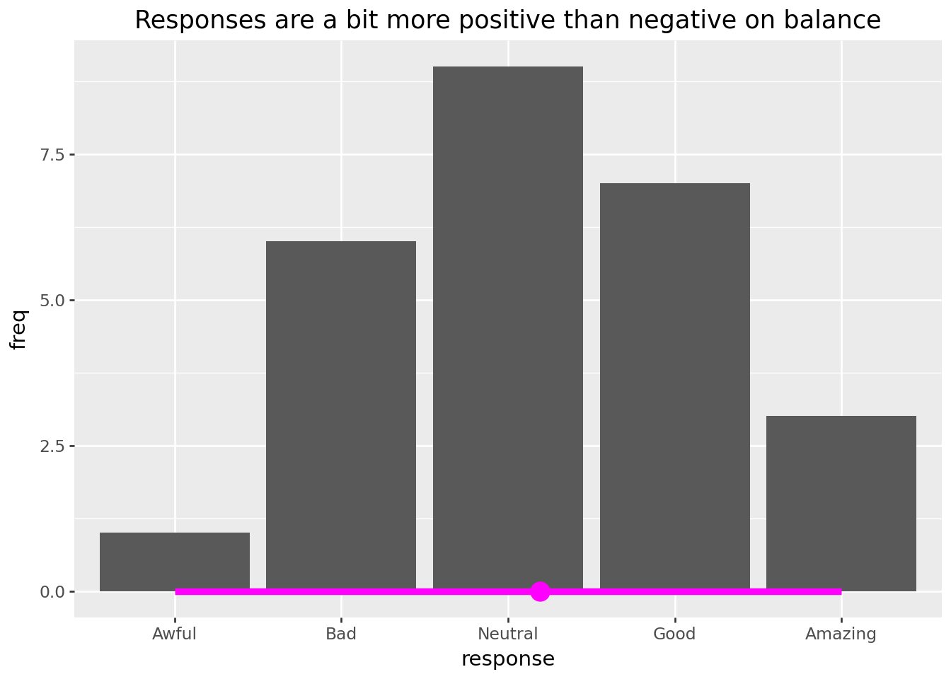
Recipe 3: geom_bal_point() and geom_support()
In the first two recipes, you defined compute that would work group-wise. In recipe #2 we briefly contrasted a panel-wise computation specification with our group-wise computation (see stat_index_panel). We saw that when introducing a categorical variable using stat_index_panel, indices were computed across the groups, instead of within groups – the behavior for stat_index.
In this recipe, we’ll use panel-wise computation throughout to look at the ‘balance’ of the frequency of discrete ordinal variables. Panel-wise compute is needed because of the discrete variable mapping, i.e. aes(x="response"). So that the data isn’t broken up by category (unique responses), we define compute_panel instead of compute_group.
Our goal is to be able to write the following code, producing the plot that follows.
survey_df = pd.DataFrame({
    "response": pd.Categorical(
        ["Awful", "Bad", "Neutral", "Good", "Amazing"],
        categories=["Awful", "Bad", "Neutral", "Good", "Amazing"],
        ordered=True,
    ),
    "freq": [1, 6, 9, 7, 3],
})

(
    ggplot(data=survey_df)
    + aes(x="response", y="freq")
    + geom_col()
    + geom_support(color="magenta", size=2)
    + geom_bal_point(color="magenta", size=7)
)
Let’s get started!
Step 0: use base plotnine to get the job done
It’s a good idea to look at how you’d get things done without extension first, just using ‘base’ plotnine. Here, we’ll plot the frequencies of some ordered responses (Awful to Amazing), and look at the ‘balance’ based on their numeric values.
import pandas as pd

from plotnine import *

survey_df = pd.DataFrame({
    "response": pd.Categorical(
        ["Awful", "Bad", "Neutral", "Good", "Amazing"],
        categories=["Awful", "Bad", "Neutral", "Good", "Amazing"],
        ordered=True,
    ),
    "freq": [1, 6, 9, 7, 3],
})

x_numeric = survey_df["response"].cat.codes.astype(int) + 1
bal_x = (x_numeric * survey_df["freq"]).sum() / survey_df["freq"].sum()
balancing_point_df = pd.DataFrame({"x": [bal_x], "y": [0]})

(
    ggplot(survey_df)
    + aes(x="response", y="freq")
    + geom_col()
    + geom_point(
        data=balancing_point_df,
        mapping=aes(x="x", y="y"),
        size=5, color="magenta",
    )
)
Step 1: Define compute. Test.
Now you are ready to begin building your extension function. The first step is to define the compute that should be done under-the-hood when your function is used. We’ll define this in a function called compute_panel_bal_point(). You will also need to include a scales argument, which plotnine uses internally. Because the x scale is converted to numeric early on in plotnine’s plot build - the compute is even simpler - you don’t need to convert your x variable to numeric as was required in Step 0!
def compute_panel_bal_point(data, scales=None):
    x_bal = (data["x"] * data["y"]).sum() / data["y"].sum()
    return data.head(1).assign(x=x_bal, y=0)
NoteYou may have noticed …
… the
scalesargument in the compute definition, which is used internally in plotnine. While it won’t be used in your test (up next), you do need it so that the computation will work in the plotnine setting.… that the compute function can only be used with data with variables
xandy. Aesthetic variable names, relevant for building the plot, are generally not found in the raw data inputs for the plot.… that we use
data.head(1).assign(...)to build the result. This preserves internal columns (likePANELandgroup) that plotnine needs for rendering. Creating a brand-new DataFrame would lose these columns.
Test compute.
(
    survey_df
    .assign(x=survey_df["response"].cat.codes + 1)
    .rename(columns={"freq": "y"})
    .pipe(compute_panel_bal_point)
)| response | y | x | |
|---|---|---|---|
| 0 | Awful | 0 | 3.192308 |
NoteYou may have noticed …
… that we prepare the data to have columns with names x and y before testing compute_panel_bal_point. Computation will fail if the names x and y are not present given our function definition. Internally in a plot, columns are named based on aesthetic mapping, e.g. aes(x="response", y="freq").
Step 2: Define new stat. Test.
Next, we define a new stat class — which will let us do computation under the hood while building our plot.
Define stat.
from plotnine.stats.stat import stat

class stat_bal_point(stat):  # <1> <2>
    REQUIRED_AES = {"x", "y"}
    DEFAULT_PARAMS = {"geom": "point"}

    def compute_panel(self, data, scales):
        return compute_panel_bal_point(data)
NoteYou may have noticed …
… that the naming convention for the stat class uses snake_case. e.g.
stat_bal_point.… that we inherit from the
statclass. In fact, your class is a subclass — you are inheriting class properties from plotnine’sstat.… that the
compute_panel_bal_pointfunction is called in thecompute_panelmethod. This means that data will be transformed panel-wise (by facet), not group-wise.… that setting
REQUIRED_AESto{"x", "y"}is consistent with compute requirements. The compute assumes data to be a DataFrame with columnsxandy. SpecifyingREQUIRED_AESin your stat can improve your user interface because standard plotnine error messages will issue when required aesthetics are not specified, e.g. “stat_bal_point()requires the following missing aesthetics:x.”
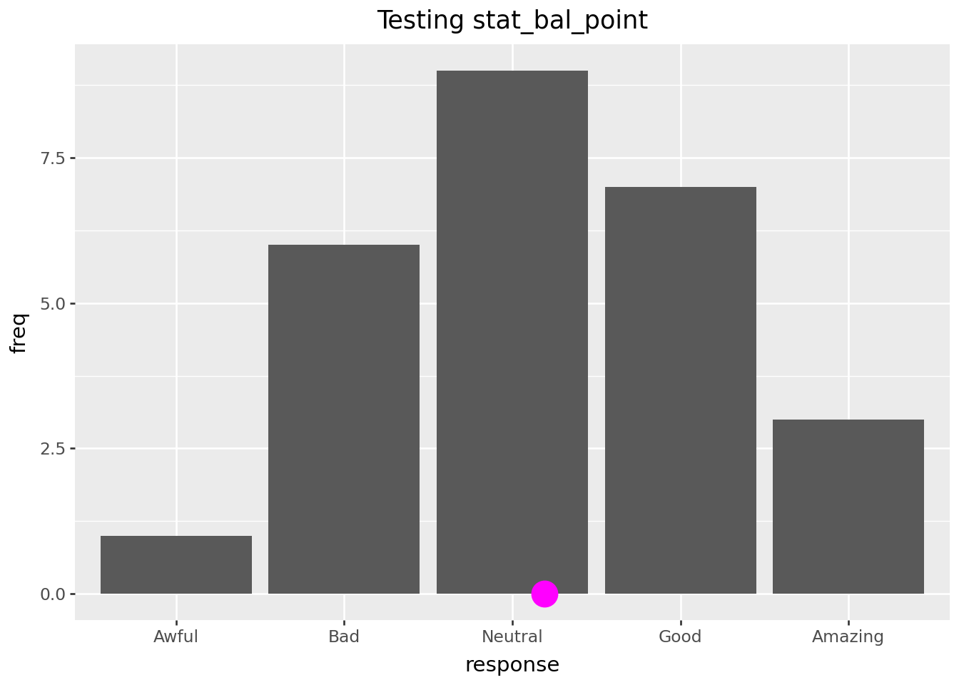
Test stat.
You can test out your stat by using it in plotnine geom_*() functions.
(
    ggplot(survey_df)
    + aes(x="response", y="freq")
    + geom_col()
    + geom_point(stat=stat_bal_point, color="magenta", size=7)
    + labs(title="Testing stat_bal_point")
)
NoteYou may have noticed …
… that we pass the class stat_bal_point to the stat argument. You could also write geom_point(stat="bal_point") which will direct to your new stat_bal_point under the hood.
TipPro tip: Think about an early exit (don’t define a user-facing function) …
You might be thinking, what we’ve done would already be pretty useful to me. Can I just use my stat as-is within geom_*() functions?
The short answer is ‘yes’! If you just want to use the stat yourself locally in a script, there might not be much reason to go on to Step 3, user-facing functions. But if you have a wider audience in mind, i.e. internal to organization or open sourcing in a package, probably a more succinct expression of what functionality you deliver will be useful - i.e. write the user-facing functions.
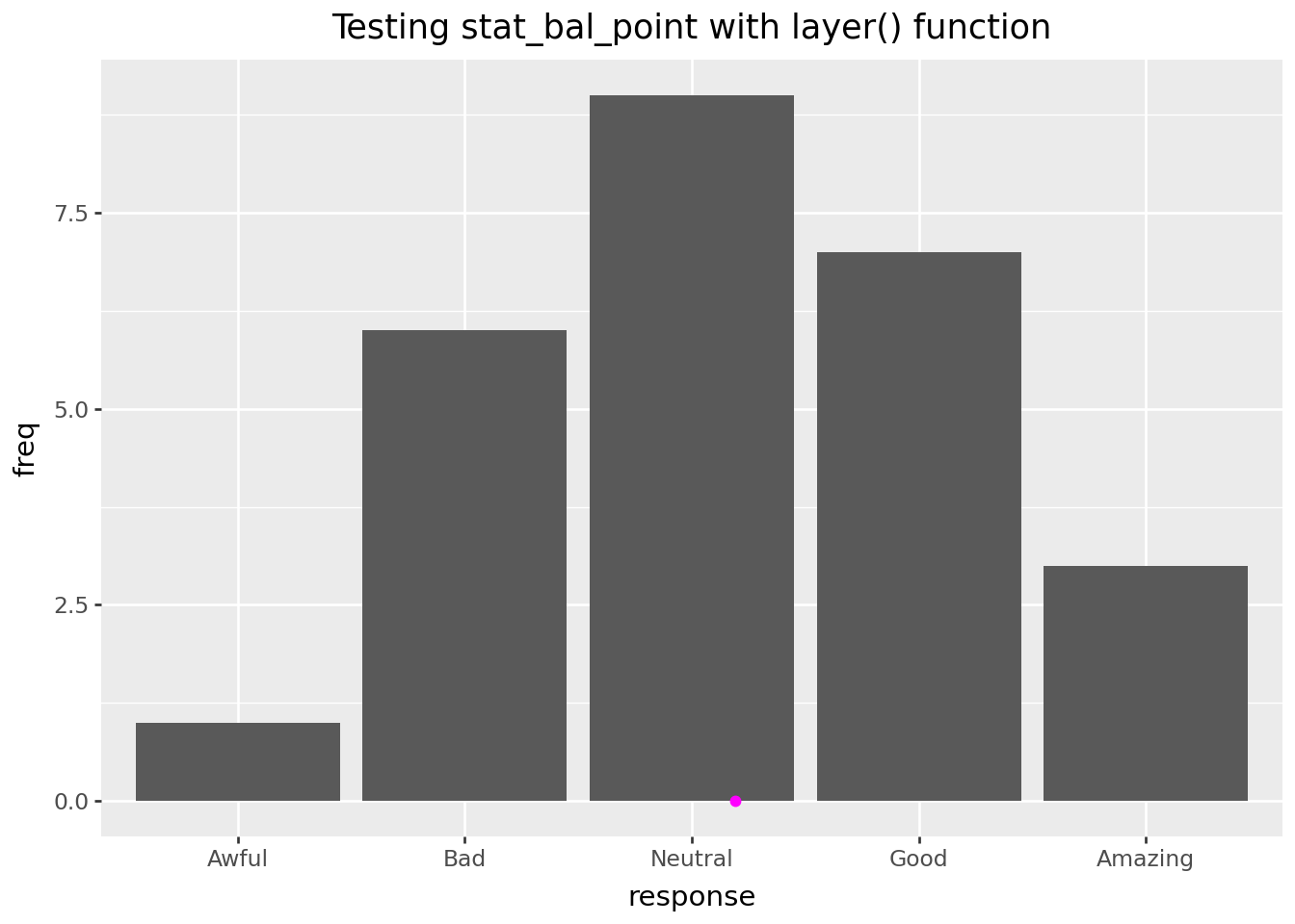
TipPro tip: consider using
layer() function to test instead of geom_*(stat=stat_new)
Instead of using a geom_*() function, you might prefer to use the layer() function in your testing step. Occasionally, you must go this route; for example, geom_vline() contains no stat argument, but you can use geom_vline in layer(). If you are teaching this content, using layer() may help you better connect this step with the next, defining the user-facing functions.
A test of stat_bal_point using this method follows. You can see it is a little more verbose, as there is no default for the position argument, and setting the size must be handled with a little more care.
from plotnine.layer import layer

(
    ggplot(survey_df)
    + aes(x="response", y="freq")
    + geom_col()
    + layer(
        geom=geom_point,
        stat=stat_bal_point,
        position="identity",
        color="magenta",
    )
    + labs(title="Testing stat_bal_point with layer() function")
)
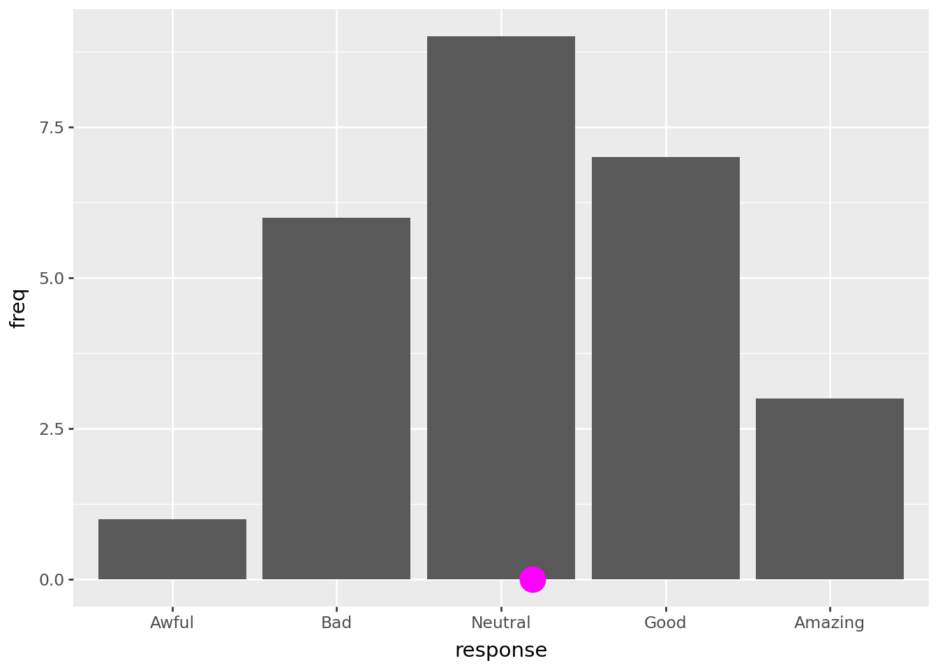
Step 3: Define user-facing functions. Test.
In this next section, we define user-facing geom_* classes. In plotnine, creating a new geom is as simple as subclassing an existing geom and setting DEFAULT_PARAMS with your new stat.
Define geom_*() class
‘Most users are accustomed to adding geoms, not stats, when building up a plot.’ ggplot2: Elegant Graphics for Data Analysis.
Because plotnine users may be more accustomed to using layers that have the geom_ prefix, you might define a geom_ class with the same properties as the stat_. Here we subclass geom_point and set the default stat to "bal_point".
class geom_bal_point(geom_point):
    DEFAULT_PARAMS = {"stat": "bal_point"}
Test/Enjoy functions
(
    ggplot(survey_df)
    + aes(x="response", y="freq")
    + geom_col()
    + geom_bal_point(color="magenta", size=7)
)
Done! Time for a review.
Here is a quick review of the classes we’ve covered, dropping tests and discussion.
NoteReview
# Step 1. Define compute
def compute_panel_bal_point(data, scales=None):
    x_bal = (data["x"] * data["y"]).sum() / data["y"].sum()
    return data.head(1).assign(x=x_bal, y=0)

# Step 2. Define stat
class stat_bal_point(stat):
    REQUIRED_AES = {"x", "y"}
    DEFAULT_PARAMS = {"geom": "point"}

    def compute_panel(self, data, scales):
        return compute_panel_bal_point(data)

# Step 3. Define geom
class geom_bal_point(geom_point):
    DEFAULT_PARAMS = {"stat": "bal_point"}
Your Turn: Write geom_support()
Using the geom_bal_point Recipe #3 as a reference, try to create a stat_support() and convenience geom_support() that draws a segment from the minimum of x to the max of x along y = 0. This might complement the geom_bal_point(), being the support upon which the data bars sit and the logical limits for the balancing point.
Hint: consider what aesthetics are required for segments. We’ll give you Step 0 this time…
Step 0: use base plotnine to get the job done
Step 1: Write compute function. Test.
Step 2: Write stat
Step 3: Write user-facing geom class.
Next up, Recipe 4: geom_cat_lm()
How would you write the function that draws residuals based on a linear model fit that contains a categorical variable, lm(y ~ x + cat)? Go to Recipe 4.