Recipe 4: geom_cat_lm(), geom_cat_fitted(), and geom_cat_residuals()
Example recipe #4: geom_cat_lm()
In this next recipe, we use panel-wise computation again to visualize a linear model that is estimated using both a continuous and a categorical variable, i.e. lm(y ~ x + cat). This may feel a bit like geom_smooth(method="lm") + aes(group="cat"). However, since geom_smooth does group-wise computation, the data is broken up before model estimation when a discrete variable is mapped like aes(color="sex") – meaning a model is estimated for each category. Let’s see how we might visualize a single model that includes a categorical variable.
Our first goal is to be able to specify a plot with newly created geom_cat_lm() (and we’ll look at defining geom_cat_fitted() and geom_cat_residuals())
(
    ggplot(penguins_clean)
    + aes(x="bill_depth_mm", y="bill_length_mm", cat="species")
    + geom_point()
    + geom_cat_lm()
)
Let’s get started!
Step 0: use base plotnine to get the job done
It’s a good idea to look at how you’d get things done without stat extension first, just using ‘base’ plotnine. The computational moves you make here can serve as a reference for building our extension function.
import pandas as pd
import statsmodels.formula.api as smf
from plotnine import *
from plotnine.data import penguins
from plotnine.layer import layer
from plotnine.session import last_plot

penguins_clean = penguins.dropna()

model = smf.ols(
    formula="bill_length_mm ~ bill_depth_mm + C(species)",
    data=penguins_clean,
).fit()

penguins_w_fitted = penguins_clean.assign(fitted=model.fittedvalues)

(
    ggplot(penguins_clean)
    + aes(x="bill_depth_mm", y="bill_length_mm", group="species")
    + geom_point()
    + geom_line(
        data=penguins_w_fitted,
        mapping=aes(y="fitted"),
        color="maroon",
    )
)
TipPro tip. Use
ggplot.layer_data() to inspect plotnine’s internal data …
Use ggplot.layer_data() to inspect the render-ready data internal in the plot. Your stat will help prep data to look something like this.
last_plot().layer_data(i=1).head() # the fitted y (not the raw data y) is of interest| y | x | group | PANEL | alpha | linetype | size | color | |
|---|---|---|---|---|---|---|---|---|
| 136 | 34.833358 | 15.5 | 1 | 1 | 1 | solid | 0.5 | maroon |
| 118 | 35.393983 | 15.9 | 1 | 1 | 1 | solid | 0.5 | maroon |
| 96 | 35.534140 | 16.0 | 1 | 1 | 1 | solid | 0.5 | maroon |
| 72 | 35.674296 | 16.1 | 1 | 1 | 1 | solid | 0.5 | maroon |
| 92 | 35.674296 | 16.1 | 1 | 1 | 1 | solid | 0.5 | maroon |
Step 1: Define compute. Test.
Now you are ready to begin building your extension function. The first step is to define the compute that should be done under-the-hood when your function is used. We’ll define this in a function called compute_panel_cat_lm(). The data input will look similar to the plot data. You will also need to include a scales argument, which plotnine uses internally.
import statsmodels.formula.api as smf

def compute_panel_cat_lm(data, scales=None):
    model = smf.ols("y ~ x + C(cat)", data=data).fit()
    return data.assign(y=model.fittedvalues)
NoteYou may have noticed …
… the
scalesargument in the compute definition, which is used internally in plotnine. While it won’t be used in your test (up next), you do need it so that the computation will work in the plotnine setting.… that the compute function can only be used with data with variables
x,y, andcat. These aesthetic variable names, relevant for building the plot, are generally not found in the raw data inputs for the plot.… that we use
C(cat)in the formula. This tells statsmodels to treatcatas a categorical variable in the model, equivalent to R’s automatic factor handling inlm().
Test compute.
## Test
(
    penguins_clean
    .rename(columns={"bill_depth_mm": "x", "bill_length_mm": "y", "species": "cat"})
    [["x", "y", "cat"]]
    .pipe(compute_panel_cat_lm)
    .head()
)| x | y | cat | |
|---|---|---|---|
| 0 | 18.7 | 39.318360 | Adelie |
| 1 | 17.4 | 37.496328 | Adelie |
| 2 | 18.0 | 38.337265 | Adelie |
| 4 | 19.3 | 40.159297 | Adelie |
| 5 | 20.6 | 41.981329 | Adelie |
NoteYou may have noticed …
… that we prepare the data to have columns with names x, y, and cat before testing compute_panel_cat_lm. Computation will fail if these names are not present given our function definition. Internally in a plot, columns are named based on aesthetic mapping, e.g. aes(x="bill_depth_mm", y="bill_length_mm", cat="species").
Step 2: Define new stat. Test.
Next, we define a new stat class — which will let us do computation under the hood while building our plot.
Define stat
from plotnine.stats.stat import stat

class stat_cat_lm(stat):  # <1> <2>
    REQUIRED_AES = {"x", "y", "cat"}
    DEFAULT_PARAMS = {"geom": "line"}

    def compute_panel(self, data, scales):
        return compute_panel_cat_lm(data)
NoteYou may have noticed …
… that the naming convention for the stat class uses snake_case. e.g.
stat_cat_lm.… that we inherit from the
statclass. In fact, your class is a subclass — you are inheriting class properties from plotnine’sstat.… that the
compute_panel_cat_lmfunction is called in thecompute_panelmethod. This means that data will be transformed panel-wise (by facet), not group-wise.… that setting
REQUIRED_AESto{"x", "y", "cat"}is consistent with compute requirements. The compute assumes data to be a DataFrame with columnsx,y, andcat. SpecifyingREQUIRED_AESin your stat can improve your user interface because standard plotnine error messages will issue when required aesthetics are not specified, e.g. “stat_cat_lm()requires the following missing aesthetics:x.”
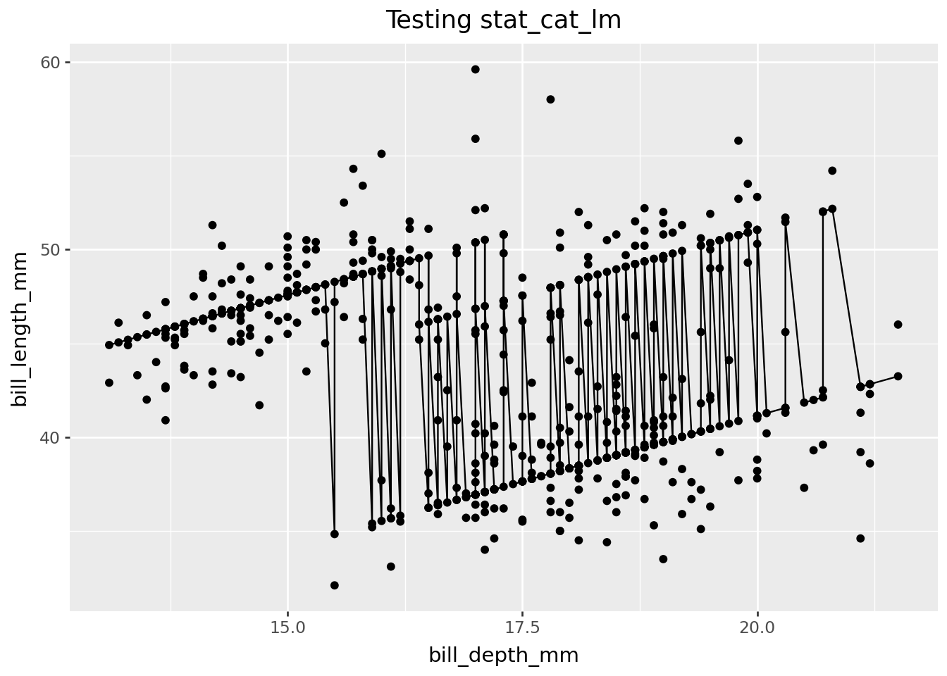
Test stat
You can test out your stat by using it in plotnine geom_*() functions.
(
    ggplot(penguins_clean)
    + aes(x="bill_depth_mm", y="bill_length_mm", cat="species")
    + geom_point()
    + geom_point(stat=stat_cat_lm)
    + geom_line(stat=stat_cat_lm)
    + labs(title="Testing stat_cat_lm")
)
NoteYou may have noticed …
… that we pass the class stat_cat_lm to the stat argument. You could also write geom_point(stat="cat_lm") which will direct to your new stat_cat_lm under the hood.
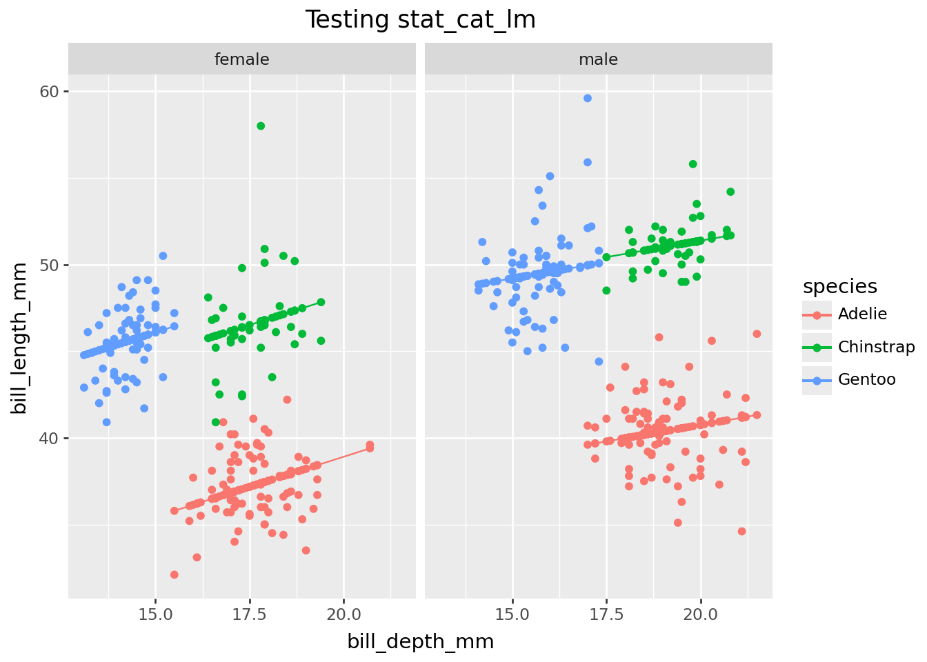
Test panel-wise behavior
(
    last_plot()
    + aes(color="species")
    + facet_wrap("sex")
)
TipPro tip: Think about an early exit (don’t define a user-facing function) …
You might be thinking, what we’ve done would already be pretty useful to me. Can I just use my stat as-is within geom_*() functions?
The short answer is ‘yes’! If you just want to use the stat yourself locally in a script, there might not be much reason to go on to Step 3, user-facing functions. But if you have a wider audience in mind, i.e. internal to organization or open sourcing in a package, probably a more succinct expression of what functionality you deliver will be useful - i.e. write the user-facing functions.
TipPro tip: consider using
layer() function to test instead of geom_*(stat=stat_new)
Instead of using a geom_*() function, you might prefer to use the layer() function in your testing step. Occasionally, you must go this route; for example, geom_vline() contains no stat argument, but you can use geom_vline in layer(). If you are teaching this content, using layer() may help you better connect this step with the next, defining the user-facing functions.
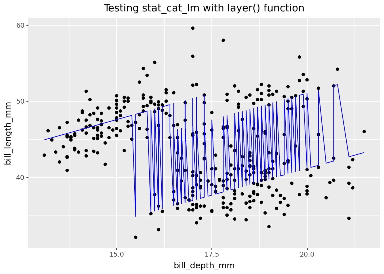
A test of stat_cat_lm using this method follows. You can see it is a little more verbose, as there is no default for the position argument, and setting the size must be handled with a little more care.
from plotnine.layer import layer

(
    ggplot(penguins_clean)
    + aes(x="bill_depth_mm", y="bill_length_mm", cat="species")
    + geom_point()
    + layer(
        geom=geom_line,
        stat=stat_cat_lm,
        position="identity",
        color="blue",
    )
    + labs(title="Testing stat_cat_lm with layer() function")
)
Step 3: Define user-facing functions. Test.
In this next section, we define user-facing geom_* classes. In plotnine, creating a new geom is as simple as subclassing an existing geom and setting DEFAULT_PARAMS with your new stat.
Define geom_*() class
‘Most users are accustomed to adding geoms, not stats, when building up a plot.’ ggplot2: Elegant Graphics for Data Analysis.
Because plotnine users may be more accustomed to using layers that have the geom_ prefix, you might define a geom_ class with the same properties as the stat_. Here we subclass geom_line and set the default stat to "cat_lm".
class geom_cat_lm(geom_line):
    DEFAULT_PARAMS = {
        "stat": "cat_lm",
        "lineend": "butt",
        "linejoin": "round",
        "arrow": None,
    }
NoteYou may have noticed…
… that
geom_cat_lminherits fromgeom_line. This means the layer will render lines by default.… that
DEFAULT_PARAMSincludes all ofgeom_line’s parameters plus"stat": "cat_lm". In plotnine,DEFAULT_PARAMSis fully replaced (not merged) when subclassing, so every parent parameter must be redeclared.
Test/Enjoy functions
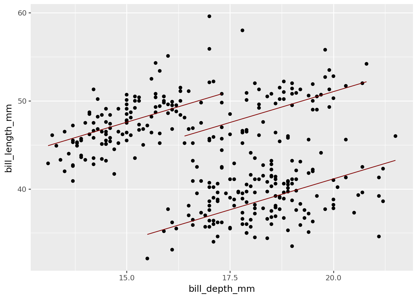
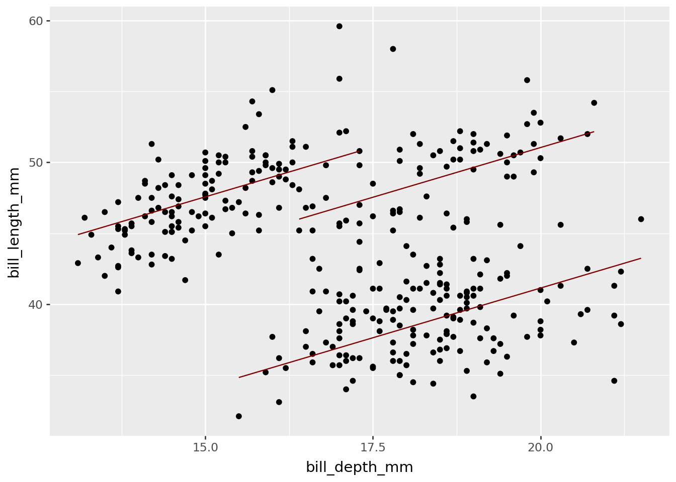
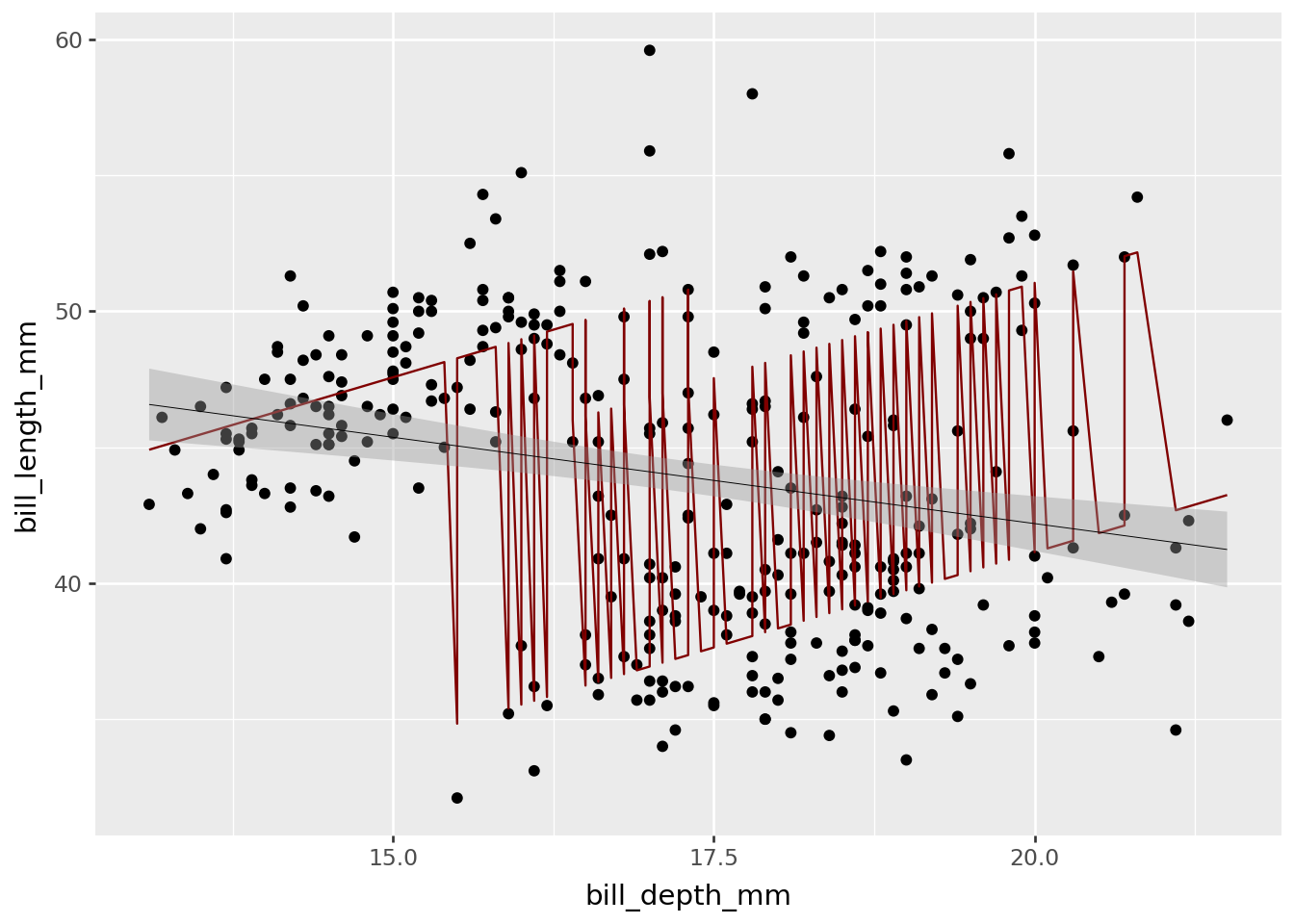
Below we use the new function geom_cat_lm(), contrasting it to geom_smooth(), which produce parallel and non-parallel slopes, respectively.
(
    ggplot(penguins_clean)
    + aes(x="bill_depth_mm", y="bill_length_mm", cat="species")
    + geom_point()
    + geom_cat_lm(color="maroon")
    + geom_smooth(method="lm", size=0.2)
)
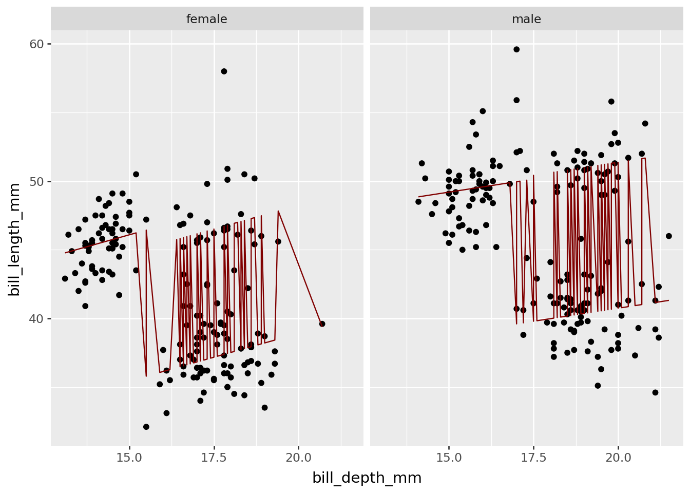
And check out conditionality
Note that because panel-wise (facet-wise) computation is specified, there are in fact, two separately estimated models for female and male. If the model is to be computed across all of the data, it’s worth considering layer-wise computation, i.e. specifying the compute_layer slot (not yet covered in these tutorials).
(
    ggplot(penguins_clean)
    + aes(x="bill_depth_mm", y="bill_length_mm", cat="species")
    + geom_point()
    + geom_cat_lm(color="maroon")
    + facet_wrap("sex")
)
Done! Time for a review.
Here is a quick review of the classes we’ve covered, dropping tests and discussion.
NoteReview
import statsmodels.formula.api as smf

# Step 1. Define compute
def compute_panel_cat_lm(data, scales=None):
    model = smf.ols("y ~ x + C(cat)", data=data).fit()
    return data.assign(y=model.fittedvalues)

# Step 2. Define stat
class stat_cat_lm(stat):
    REQUIRED_AES = {"x", "y", "cat"}
    DEFAULT_PARAMS = {"geom": "line"}

    def compute_panel(self, data, scales):
        return compute_panel_cat_lm(data)

# Step 3. Define geom
class geom_cat_lm(geom_line):
    DEFAULT_PARAMS = {
        "stat": "cat_lm",
        "lineend": "butt",
        "linejoin": "round",
        "arrow": None,
    }
Your Turn: Write geom_cat_fitted() and geom_cat_residuals()
Using the geom_cat_lm Recipe #4 as a reference, try to create a geom_cat_fitted() and geom_cat_residuals() that draws fitted values and segments between observed and fitted values for a linear model with a categorical variable.
Hint: consider what aesthetics are required for segments. We’ll give you Step 0 this time…
Step 0: use base plotnine to get the job done
Step 1: Write compute. Test.
Step 2: Write stat.
Step 3: Write user-facing geom classes.
Congratulations!
If you’ve finished all four recipes, you should have a good feel for writing stats, and stat_*() and geom_*() classes.